Last time, we went over representing natural numbers in lambda calculus, as well as addition, multiplication and exponentiation. In this post, we'll cover booleans, logical operators and pairs, which will help us define subtraction.
Typically, the boolean values true (T) and false (F) are represented as:
T = (λx,y -> x)F = (λx,y -> y)
Both are functions of two arguments, with T returning the first and F returning the second.
This lends itself very well to control flow. Try writing the if-expression (if cond a b), which returns a if cond is true and b otherwise. (We can think of if as a function that takes 3 arguments.)
(if cond a b) = (cond a b)
if is just the identity function! The way booleans are defined allows them to perform control flow by themselves: if cond is true, the first argument a is returned, otherwise the second b is returned.
Logical Operators
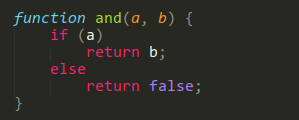
Next, let's define logical AND, OR and NOT.
(and a b) = (a b F)(or a b) = (a T b)(not a) = (a F T)
These essentially translate to how you would implement these operators in any language, e.g.
Now that we have booleans, we can express predicates, also known as conditions. One of the simplest is zero?, which tests if a natural number is equal to 0 or not.
(zero? a) = ((a F not) F)
This one is a bit of a doozy. Recall that 0 = (λx,y -> y) and e.g. 2 = (λx,y -> (x (x y))). The difference between 0 and other natural numbers is that 0 never applies the first argument, while the other numbers apply it N times. So we'd like a function that we can apply repeatedly without changing a F value (for non-zero a), with its initial value being T. The function sounds suspiciously like id, and in order to change T to F we need a NOT.
The trick is that (F x) = (λy -> y), which is id. So (F (F x)) is also id, since we can substitute x = (F x). This means we can apply F as many times as we want without changing the result from id, and if we don't apply F at all, we just have x. So the easiest way to represent 0 is to apply F to not, a times, which is then applied to F.
- When
ais 0,(0 F not) = not, so(zero? 0) = (not F) = T - When
aisn't 0,(a F not) = id, so (zero? a) = (id F) = F
Pairs
Next, we can define a pair. A pair (a, b) is represented with the function (λx -> (x a b)). Essentially, any function that wants to interact with the pair receives its components as the first two arguments.
We can construct a pair given two arguments just from the definition:
(pair a b) = (λx -> (x a b))
Of course, we'd like helper functions to read just the first and second values of the pair:
(fst p) = (p T)(snd p) = (p F)
You didn't forget about T and F, which return the first and second argument, did you?
We can now work toward the predecessor function, using pairs. If we can generate pairs (N + 1, N), then we can get the predecessor of N+1 by taking the second of that pair.
We'll first define a function phi that transforms a number a into the pair (a + 1, a).
(phi a) = (pair (succ a) a)
But we'd like to be able to call this function over and over again, so it makes more sense for the input to be a previously-generated pair (which also has the (N+1, N) shape):
(phi p) = (pair (succ (fst p)) (fst p))
Now, calling phi on (0, 0) results in (1, 0). If we called phi two times instead, that results in (2, 1). Note that the predecessor of 2 is 1. Thus, we can define:
(pred a) = (snd (a phi (pair 0 0)))
An interesting consequence is that the predecessor of 0 is 0. This will be important later.
Subtraction
We can finally define subtraction! This one should be easy to derive:
(sub a b) = (b pred a)
Remember that subtraction is non-commutative! The above is b subtracted from a, which is equivalent to calling pred on a, b times. As mentioned earlier, if the result would become negative, 0 is returned instead. Subtraction isn't closed under the natural numbers anyways.
We can use that trick to define inequalities:
(≥ a b) = (zero? (sub a b))
(< a b) = (not (≥ a b))
...etc.
and two numbers are equal iff a ≥ b and b ≥ a, so:
(= a b) = (and (≥ a b) (≥ b a))
Now we've got a lot of the basics for working with numbers. Next we'll look at expanding to integers and rationals, as well as recursion which will help us define division.